The consequence is that the friction is strongest right at the boundaries, the resulting shear stress τ_w is measured by the viscosity constant and the flow speed gradient, e.g. at wall sections parallel to the y-axis:

τ_w = η (∂ v_x/ ∂z).

In laminar flow the averaging tendency of diffusion has as consequence that the boundary layer reaches more and more into the flow and eventually dominates the velocity gradients in the whole microchannel. So the shear stress τ_w distributes eventually smoothly over the entire channel, hence we drop the index ”w” standing for ”wall”. τ also can be interpreted as the momentum flux across the lamina from the bulk towards the boundaries. This means indeed, that the moving fluid pulls the tubing towards its flow direction (a garden hose stretches out, once water is flowing through).

If we look at the change rate of this shear stress in the fluid across the channel, we obtain a number, which is surprisingly constant at any point. This is the externally applied pressure gradient along the channel which makes the fluid moving. We now understand the inner mechanics of the governing equation of a stationary flow against a pressure gradient in x-direction in a tube of arbitrary shape, which reads:

∂²v_z/∂y² + ∂²v_z/∂z² =1/η ⋅ ∂p/∂x

Note that with vanishing pressure gradient (right side) of very large viscosities this equation approaches the diffusion equation where any movement is suppressed by the boundary condition (disappearing velocity at the boundaries). This equation is a reduced Navier-Stokes equation.

For time-dependent laminar flow the left side just needs to be extended by -ρ/η ⋅ ∂ v_x / ∂t.

The most common channel geometries for microfluidic applications are cylindrical or rectangular. For cylindrical shapes the solution is a parabolic velocity profile (u_C):

u_C (r) = u₀ ( 1 – ( r/R)²)

with the maximum velocity in the center of the tubing u₀ = -R²(∂p/∂x)/(4η), the radius of the tubing (R) and the distance from the center line of the tubing (r). The negative sign indicates that the flow is oriented inverse to pressure gradients, i.e. from high to low pressures. Integration gives the total volume flow rate: Q=π R⁴ / (8 η ) ⋅ Δp/Δ x, the famous Hagen-Poiseuille law.

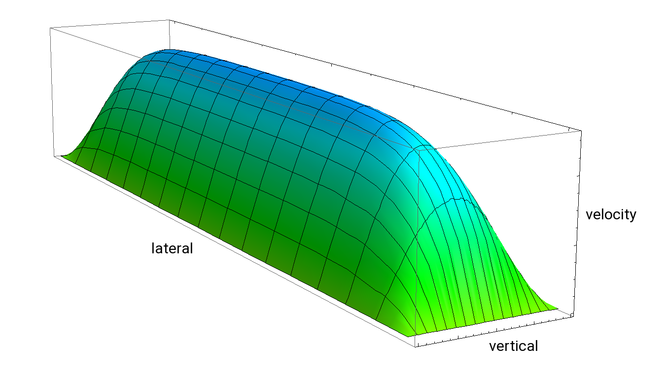
For rectangular channel profiles ranging from (- w/2 < y < + w/2) and (- h/2 < z < + h/2) with width w and height h ≤ w, the velocity profile can be obtained by solving the partial differential equation with the method of separation of variables, which can be found in the literature.[1] Now the solution consists of a series of entangled hyperbolic and trigonometric functions depending on the inverse aspect ratio w/h and y/h, z/h. It is useful to note that for small aspect ratios the lateral profile is nearly entirely flat whereas the vertical profile remains curved. This is plausible, since going to the extreme case of an infinitely wide channel, the horizontal profile becomes perfectly flat. This observation hints at a way to minimise the dispersion of small samples dissolved in a flowing carrier fluid.

A very good approximation for the total volume flow rate for the whole range from close to unity to very small aspect ratios h/w is given by:

Q = ((833 h³ w – 523 h⁴ tanh(π/2 ⋅ w/h)) / η) ⋅ Δ p / Δ x. [2]

On this website you can find a calculator for the total volume flow rate and the related pressure in cylindrical and rectangular channels. We invite you to explore different value sets and different geometries.

References:

[1] Bastian E. Rapp, Microfluidics: Modeling, Mechanics, and Mathematics (https://doi.org/10.1016/C2012-0-02230-2)

[2] Fütterer, C., Biophysical Tools GmbH

Authors: Fütterer, C., Kubitschke, H.